qBAS benchmark
qBAS protocol
The qBAS protocol was introduced by M. Benedetti et al. in [1] in 2018. The whitepaper describes the framework Data-Driven Quantum Circuit Learning (DDQCL) which evaluates the performance of quantum computers at learning probabilistic generative models. The data set model to learn for assessing the qBAS score is the Bars and Stripes (BAS) data set. This data set is easy to generate and verify for system sizes of up to a hundred qubits.
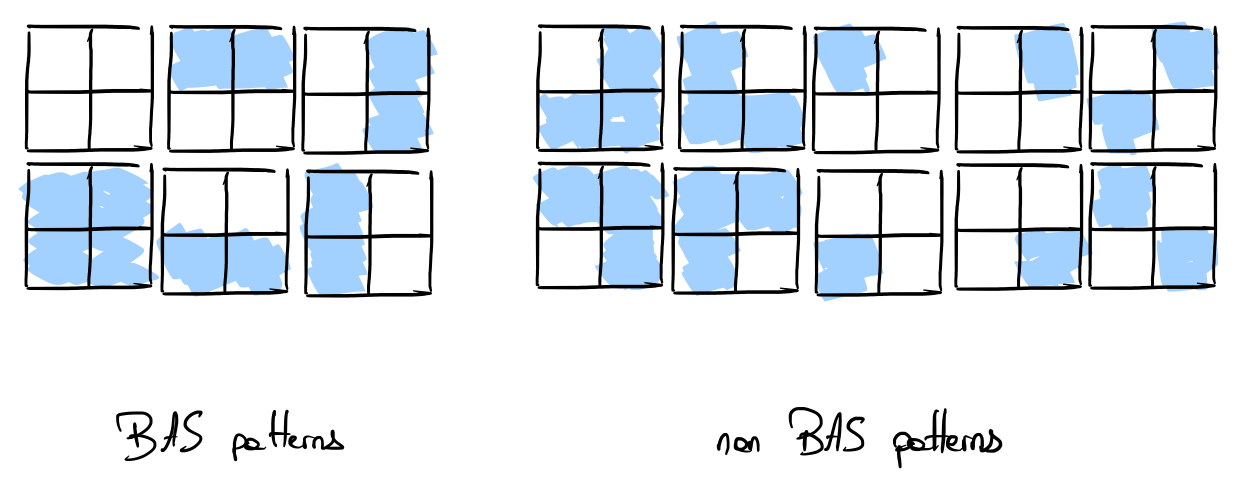
Bars and Stripes is a set of images of \(n \times m\) pixels. For a fixed value of \(n\) and \(m\), there are \(N_{BAS(n, m)}=2^n + 2^m -2\) images in the image set. The following picture shows the data set for \(n=m=2\) pixels. In this case, the optimal output distribution samples each BAS pattern with \(1/6\) probability.
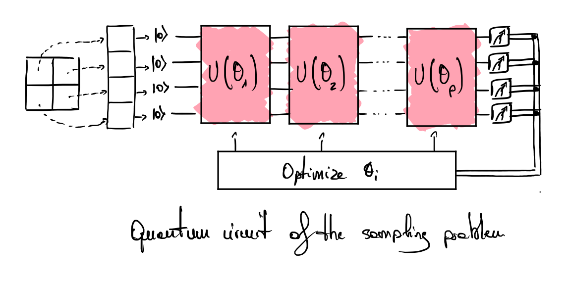
The protocol aims to evaluate the capabilities of quantum computers to uniformly sample bitstrings corresponding to each image of this set. Each pixel has a binary color (blue or white) and is associated with a qubit, which states \(\ket{0}\) and \(\ket{1}\) encode the colors. Each image should be sampled with probability \(1/N_{BAS(n, m)}\). The quantum circuit used for the evaluation is a variational circuit composed of \(p\) layers. The implementation of the layer \(U(\theta_i)\) is free but must be parameterized by a single angle \(\theta_i\). Importantly, the number of layers \(p\) is fixed and do not scale with the size of input instances (we note the list of angles to optimize \(\vec{\theta} = (\theta_1, \theta_2, ..., \theta_p)\)). The gate layout of each layer can be individually optimized to create a circuit template, but an overall compilation process that optimizes the whole circuit is not authorized.
The first step consists of learning the probability distribution of the BAS data set. A \(n_{shots}\) sampling is used to build the empirical probability of observing each bitstring constituting a BAS pattern \(x_i\). The cost function used to optimize the values of the angles \(\vec{\theta}\) is:
\[C \left(\vec{\theta} \right) = \frac{1}{N_{BAS(n, m)}} \sum_{i=1}^{N_{BAS(n, m)}} \ln \left( \max(\epsilon, P_{\vec{\theta}}(x_i)) \right)\]where the \(\epsilon\) is used to avoid cases when \(P_{\vec{\theta}}(x_i) = 0\). The reader might notice that this step does not scale favorably (some clues using other objectives to have a better scaling are given in the supplementary material of [1]).
The second step consists of estimating the qBAS-score with the optimized \(\vec{\theta}\) parameter. The aim is to evaluate the \(F_1\) score of the parametrized quantum circuit (harmonic mean between the precision and recall). The precision is the fraction of sampled states that are effectively BAS patterns. The recall corresponds to the fraction of the number of unique valid patterns \(\lvert \{ x_i \mid P_{\vec{\theta}} (x_i)>0 \} \rvert\) over the total number of unique patterns \(N_{BAS(n, m)}\). To assess this score, setting the number of samples \(n_{shots}\) is very important (otherwise, the recall can be made artificially high). The authors of [1] detail a method to estimate a reasonable number of samplings based on the coupon collector’s problem. We reproduce a table from the article that reports the number of shots that should be used for different sizes \(n\) and \(m\).
| (\(n\), \(m\)) | #qubits | \(N_{BAS(n, m)}\) | \(n_\mathrm{shots}\) |
|---|---|---|---|
| (2, 2) | 4 | 6 | 15 |
| (2, 3) | 6 | 10 | 30 |
| (3, 3) | 9 | 14 | 46 |
| (4, 4) | 16 | 30 | 120 |
| (7,7) | 49 | 254 | 1554 |
| (8, 8) | 64 | 510 | 3475 |
| (10, 10) | 100 | 2046 | 16780 |
Configuration of the experiment
- The experimental part does not mention the use of error mitigation methods.
- The structure of the circuit in completely free.
- Each layer of the quantum circuit is used as a template and is fixed.
- The number of shots to assess the qBAS score is very important and must be specified.
References
- [1]M. Benedetti, D. Garcia-Pintos, O. Perdomo, V. Leyton-Ortega, Y. Nam, and A. Perdomo-Ortiz, “A generative modeling approach for benchmarking and training shallow quantum circuits,” npj Quantum Information, vol. 5, no. 1, May 2019, doi: 10.1038/s41534-019-0157-8. [Online]. Available at: http://dx.doi.org/10.1038/s41534-019-0157-8