Fidelities and errors
Figures of Merit (FoMs) for classical probability distributions
Quantum states and processes cannot be observed directly, but measurement outcomes (i.e., bitstrings distribution) can be used as a proxy to get information about these properties. Repeating the preparation and measurement of the same quantum state results in a probability associated with each bitstring that can be observed. Quantum processes act on states, which can then be measured to extract information about these processes.
The outcome of an actual implementation can be described with a probability distribution \(\mathbf{\widetilde{p}}\) (denoted with \(\sim\) character). This distribution can be compared to the ideal target probability distribution \(\mathbf{p}\) describing the outcome of a perfect quantum processor without noisy operations. Classical figures of merit comparing probability distributions can be used to evaluate how similar or different the two distributions are. Among these FoMs, we outline those that are considered as metrics.
To be considered a metric (in the mathematical sense), a FoM \(D(\mathbf{p}, \mathbf{q})\) evaluated on distributions \(\mathbf{p}\) and \(\mathbf{q}\) must:
- be positive: \(D(\textbf{p}, \textbf{q}) \geq 0\)
- be symmetric: \(D(\textbf{p}, \textbf{q}) = D(\textbf{q}, \textbf{p})\).
- satisfy the triangle inequality: \(D(\textbf{p}, \textbf{r}) \leq D(\textbf{p}, \textbf{q}) + D(\textbf{q}, \textbf{r})\).
- be null when equality: \(D(\textbf{p}, \textbf{q}) = 0\) if and only if \(\textbf{p}= \textbf{q}\).
The reader may refer to [1] for an interesting discussion on the properties of metrics.
The next table summarizes the different FoMs that can be evaluated from the measurement outcomes. It is assumed that the probability distribution is established over \(2^n\) different possible bitstrings in \(\{0, 1\}^n\), where \(n\) denotes the number of qubits. The probability associated to each bitstring \(x\) is given by the probability distribution \(\mathbf{p}\) as \(\mathbf{p}(x)\).
| Name | Formula | Value if \(\mathbf{p} = \mathbf{\widetilde{p}}\) | Bounds | Is a metric ? | Operational interpretation |
|---|---|---|---|---|---|
| \(L_1\) distance L1 distance aka. Manhattan distance manhattan distance |
$$L_1 \left( \mathbf{\widetilde{p}}, \mathbf{p} \right) = \left\lVert \mathbf{\widetilde{p}} - \mathbf{p} \right\rVert_1$$$$ = \sum_{x \in \{0,1\}^n} \left| \mathbf{\widetilde{p}}(x) - \mathbf{p}(x) \right|$$ | 0 | $$[0, 2]$$ | yes | |
| Total variation distance Total variation distance (tvd)aka. Kolmogorov distance Kolmogorov distanceaka. Normalized \(L_1\) distance Normalized L1 distanceaka. Trace distanceTrace distance |
$$d_\mathrm{TV}\left(\mathbf{\widetilde{p}}, \mathbf{p}\right) = \frac{1}{2} L_1 \left( \mathbf{\widetilde{p}}, \mathbf{p} \right)$$ | 0 | $$[0, 1]$$ | yes | Single-shot discrimination error rate |
| Bhattacharya coefficient Bhattacharya coefficientaka. Statistical overlapStatistical overlap |
$$BC \left(\mathbf{\widetilde{p}}, \mathbf{p} \right) = \sum_{x \in \{0,1\}^n} \sqrt{\mathbf{\widetilde{p}}(x) \mathbf{p}(x)}$$ | 1 | $$[0, 1]$$ | N/M | Overlap measure between two distributions |
| Hellinger fidelity* Hellinger fidelityaka. Classical fidelityClassical fidelity |
$$F \left(\mathbf{\widetilde{p}}, \mathbf{p} \right) = \left( \sum_{x \in \{0,1\}^n} \sqrt{\mathbf{\widetilde{p}}(x) \mathbf{p}(x)} \right)^2$$ | 1 | $$[0, 1]$$ | no | |
| Hellinger distance [2]Hellinger distance | $$d_\mathrm{H}\left(\mathbf{\widetilde{p}}, \mathbf{p} \right) = \sqrt{1-\sqrt{F\left(\mathbf{\widetilde{p}}, \mathbf{p}\right)}}$$ | 0 | $$[0, 1]$$ | yes | |
| Bhattacharya distanceBhattacharya distance | $$d_\mathrm{B}\left(\mathbf{\widetilde{p}}, \mathbf{p} \right) = \frac{1}{2} \ln \left(BC \left(\mathbf{\widetilde{p}}, \mathbf{p} \right) \right)$$ | 0 | $$[0, \infty]$$ | no, do not satisfy triangle inequality | Metric measuring the overlap between two distributions |
| Kullback-Leibler deviation [3] Kullback-Leibler deviationaka. Relative entropy Relative entropy |
$$d_\mathrm{KL}\left(\mathbf{\widetilde{p}} || \mathbf{p} \right) = \sum_{x \in \{0,1\}^n} \mathbf{\widetilde{p}}(x) \log \left( \frac{\mathbf{\widetilde{p}}(x)}{\mathbf{p}(x)} \right)$$ | 0 | $$[0, \infty]$$ | no, do not satisfy triangle inequality | Many interpretations in statistics, inference … [4] |
| Entropy entropyaka. Shannon entropyShannon entropy |
$$H\left(\mathbf{p}\right) = -\sum_{x \in \{0,1\}^n} \mathbf{p}(x) \log \left(\mathbf{p}(x) \right)$$ | N/M | $$[0, \infty]$$ | N/M | |
| Cross-entropyCross-entropy | $$H(\mathbf{\widetilde{p}}, \mathbf{p}) = H\left(\mathbf{p}\right) + d_{KL}\left(\mathbf{\widetilde{p}} || \mathbf{p}\right)$$ $$= -\sum_{x \in \{0,1\}^n} \mathbf{\widetilde{p}}(x) \log \left(\mathbf{p}(x) \right)$$ | Min val of \(H(\mathbf{p}, \mathbf{\widetilde{p}})\) | $$[0, \infty]$$ | no | |
| Linear Cross-entropylinear cross-entropy | $$H_\mathrm{lin}\left(\mathbf{\widetilde{p}},\mathbf{p}\right) = 2^n \left(\sum_{x \in \{0,1\}^n} \mathbf{\widetilde{p}}(x) \mathbf{p}(x)\right) – 1$$ | 1 | $$[0, 1]$$ | no |
*Sometimes, the fidelity can be reported as the square root of the quantities reported here. We prefer this representation as it can be directly linked to the success probability of a quantum computation [1].
FoM for quantum states
The matrix density operator \(\rho=\sum_i p_i \ket{\psi_i} \bra{\psi_i}\) is used to model uncertainty about the knowledge of a quantum state. Each state \(\ket{\psi_i}\) is a pure state associated with the probability \(p_i\). We continue using the same notation where \(\rho\) (resp. \(\widetilde{\rho}\)) represents the ideal target (resp. actual implemented) density operator.
Assessing the distinguishability between quantum states strongly depends on the measures being done on the quantum states. For this reason, the measurement (Positive Operator-valued Measure) maximizing the distinguishability between the two quantum states \(\rho\) and \(\widetilde{\rho}\) is always chosen. In this way, results obtained from these measurements are used to build FoMs that assess an upper bound on the error rate of a measurement done on the quantum state. These FoMs can be used to evaluate the performance of state preparations.
In the following table, the trace operator \(\Tr\) on a matrix \(A\) is defined as : \(\Tr(A) = \sum_{i} a_{ii}\).
| Name | Formula | Value if \(\mathbf{\rho = \widetilde{\rho}}\) | Bounds | Is a metric ? | Operational interpretation |
|---|---|---|---|---|---|
| Trace distance [5]Trace distance | $$d_{tr} \left(\widetilde{\rho}, \rho \right) = \frac{1}{2} \left\lVert \widetilde{\rho} - \rho \right\rVert_1$$$$= \frac{1}{2} \Tr \left|\widetilde{\rho} - \rho \right|$$ | 0 | $$[0, 1]$$ | yes | inherits properties from classical total variation distance |
| State fidelity [5] (two pure states)State fidelity |
$$\widetilde{\rho} =\ket{\psi}\bra{\psi}, \rho =\ket{\phi}\bra{\phi}$$$$F\left(\widetilde{\rho}, \rho\right) = |\braket{\psi | \phi}|^2$$ | 1 | $$[0, 1]$$ | no | Proxy to success probability of a quantum computation |
| State fidelity [5] (target is pure) (the other is mixed) |
$$\widetilde{\rho} = \sum_i p_i \ket{\psi_i} \bra{\psi_i}, \rho =\ket{\phi}\bra{\phi}$$$$F\left(\widetilde{\rho}, \rho\right) = \braket{\phi | \widetilde{\rho} | \phi} = \Tr \left(\widetilde{\rho} \ket{\phi}\bra{\phi} \right)$$ | 1 | $$[0, 1]$$ | no | Proxy to success probability of a quantum computation |
| State fidelity* [5] (with two mixed states) |
$$F \left(\widetilde{\rho}, \rho \right) = \left( \Tr \sqrt{\sqrt{\widetilde{\rho}} \rho \sqrt{\widetilde{\rho}}} \right)^2$$ | 1 | $$[0, 1]$$ | no | Proxy to success probability of a quantum computation |
| Bures distance [1] (finite version of Bures metric)Bures distance |
$$B \left( \widetilde{\rho}, \rho \right) = \sqrt{2-2\sqrt{F \left( \widetilde{\rho}, \rho \right)}}$$ | 0 | $$[0, \sqrt{2}]$$ | yes | Turn the fidelity to a euclidean distance between two pure states |
| Bures angle [1] aka. quantum angle Bures angle |
$$A \left( \widetilde{\rho}, \rho \right) = \arccos \sqrt{F \left( \widetilde{\rho}, \rho \right)}$$ | 0 | $$[0, 2\pi]$$ | yes | Turn the fidelity to an angle between two pure states |
| State infidelityState infidelity | $$\epsilon_{inf} = 1-F$$ | 0 | $$[0, 1]$$ | yes | Proxy to failure probability of a quantum computation |
| Quantum relative entropy [5]Quantum relative entropy | $$S \left(\widetilde{\rho} || \rho \right) = \Tr \left( \widetilde{\rho} \log(\widetilde{\rho}) \right) - \Tr \left( \widetilde{\rho} \log \left( \rho \right) \right)$$ | 0 | $$[0, \infty]$$ | no, do not satisfy triangle inequality |
*Sometimes, the fidelity can be reported as the square root of the quantities reported here. We prefer this representation as it can be directly linked to the success probability of a quantum computation [1].
FoM for quantum processes
Quantum processes (gates) define operations that transform the quantum state to another quantum state. These operations need to be accurate, and FoMs have been defined to measure the quality of implementation of these processes. The evolution of the noisy quantum computer can be described with two main components:
- The quantum state: the system of interest used in the computation \(\rho\).
- The environment in which the quantum state evolves \(\rho_{env}\).
The evolution of the quantum state can be seen as a joint evolution of the state of interest \(\rho\) and its environment \(\rho_{env}\) (see figure reproduced from [6]). This evolution can be described by a single unitary \(U\) acting over both systems. At the end of the evolution, the quantum state \(\rho\) is measured using a projective measurement, which consists in a partial trace over the environment.
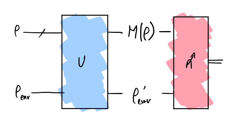
The map \(\rho \rightarrow M(\rho)\) represents a quantum operation if it is a Complete Positive Trace Preserving (CPTP) map. CP means that \(M(\rho)\) must be positive semi-definite (i.e., no output with a negative probability). TP means that each measurement outcome probability adds up to 1. The reader may refer to [6] for a pedagogical introduction and discussion on CPTP.
Benchmarking quantum processes involves comparing ideal implementations of the map \(M\) to the actual implementation \(\widetilde{M}\). In general, these maps are directly called quantum gates.
| Name | Formula | Value if \(\rho = \widetilde{\rho}\) | Bounds | Is a metric ? | Operational interpretation |
|---|---|---|---|---|---|
| Diamond distance [7] [8] Diamond distance | $$d_\mathrm{\diamond} \left(\widetilde{M}, M \right) = \frac{1}{2} \left\lVert \widetilde{M}-M \right\rVert_\mathrm{\diamond} $$$$ = \max_\rho \left\lVert (\widetilde{M} \otimes I)\rho - \left(M \otimes I \right) \rho \right\rVert_1$$ | 0 | $$[0, 1]$$ | no | Achievable upper bound on the probability of distinguishing \(M\) from \(\widetilde{M}\) |
| Jamiołkowski trace distance [9] [1]Jamiołkowski trace distance | $$d_\mathrm{tr\_J}\left(\widetilde{M}, M \right) = \frac{1}{2} \left\lVert \left(\widetilde{M}_A \otimes I_B - M_A \otimes I_B \right) \ket{\psi_{AB}} \bra{\psi_{AB}} \right\lVert_1$$ | 0 | $$[0, 1]$$ | yes | Provide a lower bound on \(d_\mathrm{\diamond}\) |
| Average gate fidelity [5]Average gate fidelity | $$F_\mathrm{avg} \left (\widetilde{M}, M \right) = \int F \left( \widetilde{M}( \ket{\psi} \bra{\psi}), M(\ket{\psi} \bra{\psi}) \right) \mathrm{d} \psi$$ | 0 | $$[0, 1]$$ | no | Inherits quantum state fidelity properties Averaged over Haar measure Used in RB |
| Average gate infidelity Average gate infidelityaka. Average error rate*Average error rate |
$$\epsilon_{r} \left(\widetilde{M}, M \right) = 1 - F_\mathrm{AVG} \left(\widetilde{M}, M \right)$$ | 1 | $$[0, 1]$$ | no | error rate |
| Entanglement fidelity [10] Aka. Process fidelityEntanglement fidelityProcess fidelity |
$$F_e \left(\widetilde{M}, M \right) = F \left( (\widetilde{M} \otimes I) ( \ket{\psi} \bra{\psi}), \left( M \otimes I \right)(\ket{\psi} \bra{\psi}) \right)$$ | 0 | $$[0, 1]$$ | no | Inherits quantum state fidelity properties |
| Entanglement infidelityEntanglement infidelity | $$\epsilon_{e} \left(\widetilde{M}, M \right) = 1 – F_\mathrm{e} \left(\widetilde{M}, M \right)$$ | 1 | $$[0, 1]$$ | no | error rate |
| Stabilized minimum fidelity [1]Stabilized minimum fidelity | $$F_\mathrm{stab} \left( \widetilde{M}, M \right) = \min_{\psi_{AB}} F \left( \left( \widetilde{M}_A \otimes I_B \right) (\ket{\psi} \bra{\psi}, \left( M_A \otimes I_B \right)(\ket{\psi} \bra{\psi}) \right)$$ | 0 | $$[0, 1]$$ | no | Inherits quantum state fidelity properties |
*The average gate infidelity is often called the average gate error rate. However, in some cases, a distinction is made between these two quantities, as in quantum error correction for rigorously linking the error correction threshold to the average gate infidelity [11].
Extra references
For further reading on error measures of quantum states and quantum processing, the reader may refer to [1]. A nice recent tutorial discusses most of these FoMs [6]. The reader can also refer to [5] for an introduction on distance measures.
References
- [1]A. Gilchrist, N. K. Langford, and M. A. Nielsen, “Distance measures to compare real and ideal quantum processes,” Physical Review A, vol. 71, no. 6, June 2005, doi: 10.1103/physreva.71.062310. Available at: http://dx.doi.org/10.1103/PhysRevA.71.062310
- [2]E. Hellinger, “Neue Begründung der Theorie quadratischer Formen von unendlichvielen Veränderlichen.,” Journal für die reine und angewandte Mathematik, vol. 1909, no. 136, pp. 210–271, July 1909, doi: 10.1515/crll.1909.136.210. Available at: http://dx.doi.org/10.1515/crll.1909.136.210
- [3]S. Kullback and R. A. Leibler, “On Information and Sufficiency,” The Annals of Mathematical Statistics, vol. 22, no. 1, pp. 79–86, Mar. 1951, doi: 10.1214/aoms/1177729694. Available at: http://dx.doi.org/10.1214/aoms/1177729694
- [4]Wikipedia, “Kullback–Leibler divergence interpretations.” 2025. Available at: https://en.wikipedia.org/wiki/Kullback%E2%80%93Leibler_divergence#Interpretations
- [5]M. A. Nielsen and I. L. Chuang, Quantum computation and quantum information. Cambridge university press, 2010.
- [6]A. Hashim et al., “Practical Introduction to Benchmarking and Characterization of Quantum Computers,” PRX Quantum, vol. 6, no. 3. APS, p. 030202, 2025.
- [7]A. Y. Kitaev, “Quantum computations: algorithms and error correction,” Russian Mathematical Surveys, vol. 52, no. 6, pp. 1191–1249, Dec. 1997, doi: 10.1070/rm1997v052n06abeh002155. Available at: http://dx.doi.org/10.1070/RM1997v052n06ABEH002155
- [8]D. Aharonov, A. Kitaev, and N. Nisan, “Quantum circuits with mixed states,” in Proceedings of the thirtieth annual ACM symposium on Theory of computing, 1998, pp. 20–30.
- [9]A. Jamiołkowski, “Linear transformations which preserve trace and positive semidefiniteness of operators,” Reports on Mathematical Physics, vol. 3, no. 4, pp. 275–278, Dec. 1972, doi: 10.1016/0034-4877(72)90011-0. Available at: http://dx.doi.org/10.1016/0034-4877(72)90011-0
- [10]B. Schumacher, “Sending entanglement through noisy quantum channels,” Physical Review A, vol. 54, no. 4, p. 2614, 1996.
- [11]Y. R. Sanders, J. J. Wallman, and B. C. Sanders, “Bounding quantum gate error rate based on reported average fidelity,” New Journal of Physics, vol. 18, no. 1, p. 012002, Dec. 2015, doi: 10.1088/1367-2630/18/1/012002. Available at: http://dx.doi.org/10.1088/1367-2630/18/1/012002