Boson Sampling
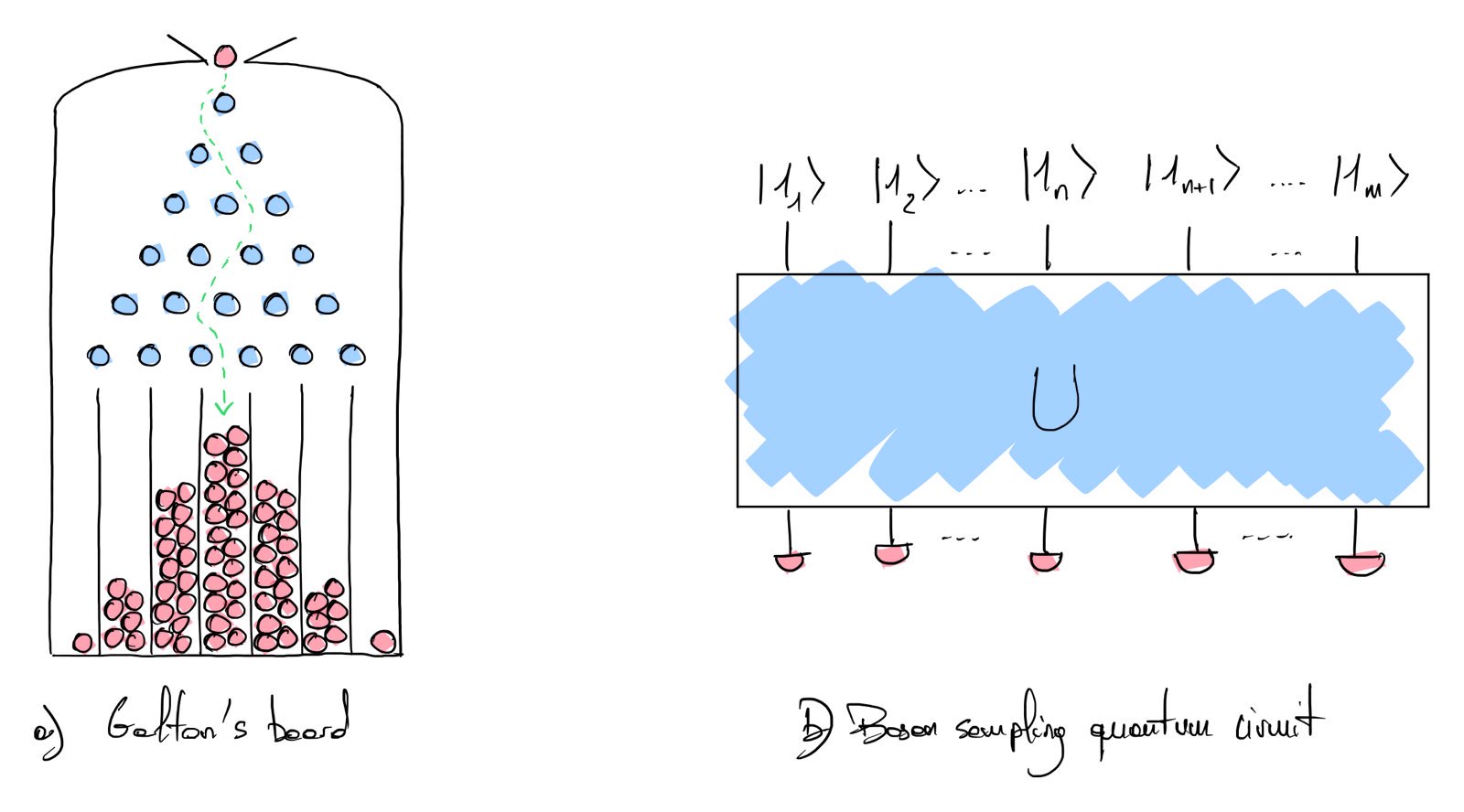
The first protocol defining the boson sampling experiment was proposed by S. Aaronson and A. Arkhipov [1]. In this article, the authors use a nice analogy to explain the concept of the boson sampling experiment. This analogy is Galton’s board (see Fig. a), which illustrates the convergence of the binomial law. This experiment comprises a board with pegs on it (blue circles). A ball (red circles) is successively introduced in the upper part of the board. When the ball falls on a peg, it has half probability of falling right and half probability falling on the left. At the end, we look at the number of balls in each column of the board. The repetition of this experiment leads to the experimental sampling of the probabilistic law determined by the arrangement of the pegs (in our case, the binomial law).
In the boson sampling experiment, a photon is used instead of the ball (see Fig. b). The track where the photon is located is called the mode (vertical lines in the Fig. b). At the end of the circuit execution, a photon in a specific mode is detected with a photon detector for each mode (red half disc Fig. b). Different detectors can be used depending on the protocol. The simplest one detects the presence or absence of photons and is called a single photon detector. A more elaborated device, the photon-number-resolving detector, counts the number of photons in each mode. It is useful in cases where collisions might happen.
We denote by \(n\) the number of photons and \(m\) the number of modes. If a single photon is used with two modes, the state corresponding to a photon in the first mode (one photon at index 1) and no photon in the second mode (zero photon at index 2) is \(\ket{1_{1}, 0_{2}}\).
The evolution of the quantum circuit is described with a random unitary matrix \(U \in \mathbb{C}^{m \times m}\) with complex coefficients. This matrix can be efficiently implemented using basic linear optic gates, including beam splitters and phase shifters. In contrast with the classical experiment using Galton’s board, estimating the output probability distribution of a complex coefficient matrix requires the computation of the permanent of the unitary \(U\) [2] (which is hard to approximate in polynomial time for classical algorithms). The approximation tends to find a probability distribution \(q\) close to the output probability distribution of the unitary matrix \(p\). The total variation distance is used to measure the closeness of both probability distributions.
We present the initial formulation of the boson sampling protocol followed by a discussion on the variations of this protocol introduced by the Scattershot Boson Sampling (SBS) protocol and Gaussian Boson Sampling (GBS) protocol.
Boson Sampling Protocol
The details of the protocol with rigorous proofs are developped in [1]. The analysis conducted in the paper assumes that the number of modes is much larger than the number of photons in the system (\(m=O(n^2)\)). It avoids collisions and finding multiple photons at the same location when the process ends. The initial state is assumed to be the deterministic Fock state with a single photon in the first \(n\) modes of the \(m\) modes: \(\ket{1_{1}, 1_{2}, ..., 1_{n}, 0_{n+1}, 0_{n+2}, ..., 0_{m}}\).
The quantum circuit is only composed of beam splitters and phase shifters. The circuit is generated to implement a unitary transformation \(\mathbb{C}^{m \times m}\) that is randomly drawn according to the Haar measure (the reader might refer to this nice article on Haar-random unitaries [3]). The depth of the circuit is of order \(O(n \log(m))\).
For this protocol, using a threshold photon detector working at room temperature is sufficient as the collision probability between photons is assumed to be very low.
We list here several issues (discussed by S. Aaronson in [4]) related to this protocol that might impact the classical simulation difficulty:
- The condition \(m = O(n^2)\) is usually not respected in practise.
- Single-photon sources are nondeterministic and hence, building the initial Fock state required by this protocol is not practical. The initialization does not scale well with the size of the problem.
- This protocol assumes that there is no photon loss, which is not the case in most practical experiments.
- This protocol does not provide tools to verify the result of the experiment.
Scattershot Boson Sampling Protocol
The Scattershot Boson Sampling experiment was motivated by the experimental limits of preparing the initial Fock state described above. This protocol has been simultaneously proposed by A. P. Lund et al. and in the blog of S. Aaronson [5], [6]. They propose to use Spontaneous Parametric Down-Conversion (SPDC) photon sources to generate the input of the quantum circuit. SPDC sources produce photons by pairs. When a pair of single photons is produced, one photon of the pair is used to herald the creation of the other photon. This can be done by detecting and absorbing the first photon. The behavior is the same when the SPDC source produces more than one pair of photons. If the SPDC source has a probability \(p\) of producing a single photon, then the probability of producing \(n\) single photons on the first \(n\) modes with independent sources would scale as \(O(p^n)\), which is a very big issue if we are looking for a quantum advantage as \(p\) is usually quite small for SPDC. The idea is to put in parallel many SPDC to have a small chance at each time step, few SPDC produce at least a single photon.
Using this protocol, the instances generated conserve the hardness clause used in the initial protocol, even if the source produced more than one pair of photons. However, in this case, it requires a photon-number-resolving detector to effectively determine the input and output state. The depth of the optical network is slightly increased to \(O(m \log(m))\).
Gaussian Boson Sampling Protocol
Gaussian Boson Sampling has been proposed by Hamilton et al. [7] and provide easier experimental possibilities. In this protocol, the initial state is a gaussian state called Single Mode Squeezed State (SMSS). The change in the initial state changes the output sampling probability, which can now be determined by computing the Hafnian of the Unitary matrix [8] (instead of the permanent). This task is also proven difficult for classical computers (\(\#P\)-complete). In this experiment, the detection is based on using photon-number-resolving detectors.
An alternative to Gaussian Boson Sampling using threshold detector was proposed in [9]. At each sample, the number of modes in which at least one photon is detected is denoted \(N_m\). The best classical algorithm to simulate gaussian boson sampling with a threshold detector scales as \(O(m^2 2^{N_m})\). This scaling shows that avoiding collisions (and hence maximizing the value \(2^{N_m}\)) is crucial to preserve the hardness of the sampling task.
Boson sampling libraries and tutorial
- Xanadu Walrus (classical library emulating Boson sampling)
- Quandela tutorial notebook (GBS)
- Xanadu tutorial notebook (BS)
Some extra references
The reader can refer to [10] for a nice introduction on Boson sampling. The blog of S. Aaronson contains many interesting discussions on the subject [11].
References
- [1]S. Aaronson and A. Arkhipov, “The computational complexity of linear optics,” in Proceedings of the forty-third annual ACM symposium on Theory of computing, 2011, pp. 333–342.
- [2]Wikipedia, “Computing the permanent.” 2025. Available at: https://en.wikipedia.org/wiki/Computing_the_permanent
- [3]O. Di Matteo, “Understanding the Haar measure.” 2021. Available at: https://pennylane.ai/qml/demos/tutorial_haar_measure
- [4]S. Aaronson, “Quantum Supremacy via Boson Sampling: Theory and Practice | Quantum Colloquium.” 2021. Available at: https://www.youtube.com/watch?v=jhBeK9y6DCo
- [5]A. P. Lund, A. Laing, S. Rahimi-Keshari, T. Rudolph, J. L. O’Brien, and T. C. Ralph, “Boson sampling from a Gaussian state,” Physical review letters, vol. 113, no. 10, p. 100502, 2014.
- [6]S. Aaronson, “Scattershot BosonSampling: A new approach to scalable BosonSampling experiments.” 2013. Available at: https://scottaaronson.blog/?p=1579
- [7]C. S. Hamilton, R. Kruse, L. Sansoni, S. Barkhofen, C. Silberhorn, and I. Jex, “Gaussian boson sampling,” Physical review letters, vol. 119, no. 17, p. 170501, 2017.
- [8]Wikipedia, “Hafnian.” 2025. Available at: https://en.wikipedia.org/wiki/Hafnian
- [9]N. Quesada, J. M. Arrazola, and N. Killoran, “Gaussian boson sampling using threshold detectors,” Physical Review A, vol. 98, no. 6, p. 062322, 2018.
- [10]B. T. Gard, K. R. Motes, J. P. Olson, P. P. Rohde, and J. P. Dowling, “An introduction to boson-sampling,” in From atomic to mesoscale: The role of quantum coherence in systems of various complexities, World Scientific, 2015, pp. 167–192.
- [11]S. Aaronson, “shtetl-Optimized.” 2005. Available at: https://scottaaronson.blog/