Quantum simulation

1. Quantum simulation with digital quantum computer (IBM)

In [1], Y. Kim et al. assess the potential of IBM quantum computers at solving quantum simulation problem with a digitial implementation of a continuous-time hamiltonian evolution. Let the IBM hardware graph (heavy hexagonal topology) defined as a set of vertices and edges\(G = (V, E)\). The Hamiltonian of interest is defined from the heavy hexagonal topology:

The aim of the experiment is to sample the output distribution of the trotterized evolution of the above Hamiltonian. The weight \(J\) is judiciously chosen so that each \(\sigma^z\sigma^z\) can be implemented with only a single CNOT gate (hence minimizing the noise induced by these gates). The weight \(h\) is related to the parameter \(\theta_h\) which parametrizes the rotation-x gates of the quantum circuit. For a fixed number of Trotter step \(T\), a corresponding circuit is built and the average value of pre-defined observables are measured with different values for the \(\theta_h\) parameter. As the circuit is built over the heavy hexagonal topology (which is a graph with maximum degree 3), a single trotter step can be done with 3 CNOT depths (see Fig. 1 and 2).

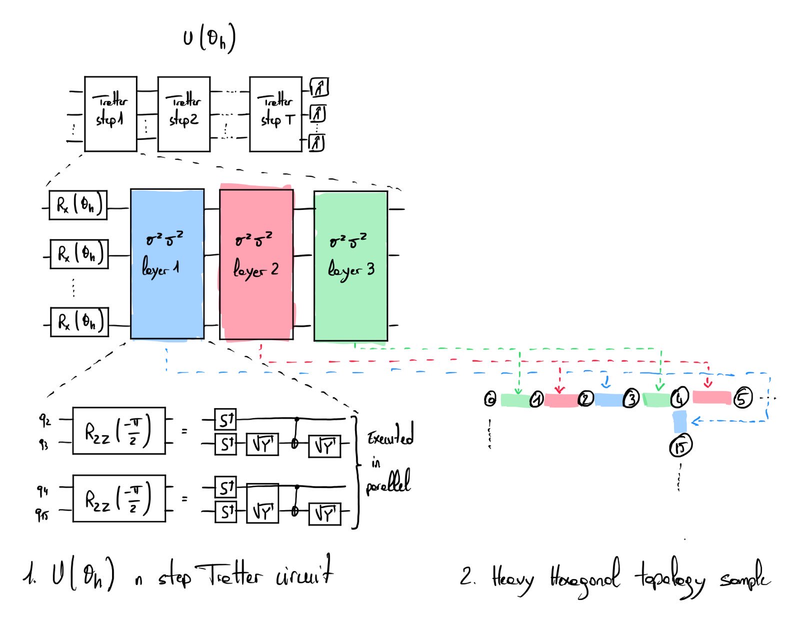
The observables are defined as weight-x observable where the x correspond to the number of qubits involved in the observable. For example, a weight-4 observable defined as (\(X_{1, 2}Y_{4}Z_{3}\)) denote that qubits 1 and 2 are measured in X basis, qubit 4 in Y basis and qubit 3 in Z basis. The experiment uses Zero-Noise Extrapolation (ZNE) method to mitigate the quantum noise.

The first benchmark consits in evaluating the behavior of quantum circuits on verifiable instances (using only Clifford circuits by setting \(\theta_h = \frac{\pi}{2})\). The second benchmark involves non-clifford circuits but choosing observables that are exactyl verifiables classically. The thrid experiment uses non-clifford circuits beyond the verifiable regime, with weight-17 observables and 5 Trotter steps in a first case, and single qubit magnetization with 20 Trotter steps in the seconde case.

The performance comparison is done with Matrix Product States methods and Isometric Tensor network states which appear to have large prohibitive costs for large instances. For the third experiment, results were obtained with the quantum computer in 8h for each individual data point \(\theta_h\) for the specified weight-17 observable. The weight-1 average magnetization was measured in 4h for each inidividual data point \(\theta_h\). The authors mention that the global processing time could be reduced to 5 minutes (by drastically reducing the classical processing time).

1.1 Belief propagation tensor network method (Refutation 1)

In [2], J. Tindall et al. propose a tensor network method using belief propagation to refute the quantum advantage claim. They build a tensor network with the same connectivity as the Heavy Hexagon lattice and employ belief propagation to contract and approximate the quantum evolution (using treelike correlations present in the wave function). They reproduce the small size results showing that their method provide better approximation of both magnetization, weight-10 and weight-17 observables than the quantum computer. They also reproduce the results of non verifiable regime with weight-1 and weight-17 observables. The results were calculated with a single laptop CPU core.

The tensor network method has been implemented on the open source library [3] and the data generated is available in [4].

1.2 Results reproduction with smaller systems

In [5], K. Kechedzhi et al. show that the results obtained for the weight-17 observable can be reproduced with smaller-size systems, having only 30 qubits. It is also showed that this new system can be simulated classically using a single GPU with only few seconds of processing time.

1.3 Clifford perturbation theory (Refutation 2)

In [6], T. Begusic et al. show the results of the initial experiment can be reproduced using sparse Pauli dynamics (called SPD in the paper). Their method use between 1 and 2 minutes of a single core of CPU to reproduce each point of the weight-1 and weight-17 observables that constitute de claim of IBM.

The same authors provided an additional work using Projected Entangled Pair Operators (PEPS) method to emulate the quantum computer [7]

1.4 Projective Entangled Pair Operator (Refutation 3)

In [8], H-J Liao et al. reproduce the results of the initial experiment using Projective Entangled Pair Operator in 3 seconds.

2. Quantum simulation with quantum annealing (D-Wave)

In [9], A. D. King et al. establish a protocol to assess the computational supremacy of D-Wave systems. These systems are analog based quantum computer (a paradigm a bit different compared to gate-based quantum computers). An example of the qubit layout is shown in Fig. 1. where each qubit is represented by a node and each programmable coupler is represented by an edge.

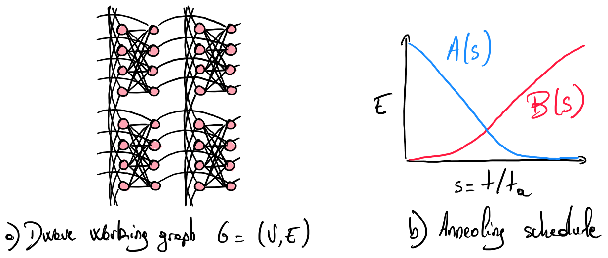
The evolution of such system can be described with a Hamiltonian operator linearly interpolating two Hamiltonians: an initial Hamiltonian \(H_\mathrm{I}\) that dominates the evolution at the beginning (\(A(0) \gg B(0)\)) and a final Hamiltonian \(H_\mathrm{F}\) that dominate the end of the evolution \(H_\mathrm{F}\) (\(B(1) \gg A(1)\)). The annealing fraction \(s = t/t_\mathrm{a}\) is expressed according to the current and total annealing time \(t\) and \(t_\mathrm{a}\) :

In the supremacy experiment, the annealing time is chosen to be really short: \(t_a \in {7, 20}\)ns. The aim of the experiment is to show that the sampling of the output distribution of the quantum computer is hard to reproduce classically. The principal figure of merit used in this experiment is the correlation error \(\epsilon_c\) defined as:

where \(c_{i,j} = \braket{\sigma_i^z \sigma_j^z}\) denotes the two-point correlation function computed for the \(n(n-1)\) couples of qubits (i.e., local and non local correlations).

For small instances (\(n \leq 64\)) the results generated by the quantum computer are verified and validated with ideal classical simulations (using Matrix Product State method). Beyond this regime, the output of the quantum computer is checked to comply with theoretical results of quantum mechanics (i.e., by estimating the Binder cumulant and showing that its value decreases with a power law of the Kibble-Zurek exponent). Each instance is run with low precision coupling weights \(J_{i,j} \in \{-1, 1\}\) and high precision coupling weights \(J_{i,j} \in \{-\frac{128}{128}, -\frac{127}{128}, ..., 0, ..., \frac{127}{128}, \frac{128}{128}\}\).

The classical methods used for comparison are:

• Matrix Product States (MPS)
• Projected Entangled-pair States (PEPS)
• Neural Quantum States (NQS)

The list of instances evaluated is presented in the following table:

Concerning the study of the runtime of classical computers, A. D. King et al. evaluate the time and comptutational space required by Matrix Product State method to match their results. They conclude that such method would take millions of years using Frontier supercomputer. They do not extensively benchmark the PEPS method using the argument that this method does not reach a sufficiently suitable correlation threshold with a descent scaling.

2.1 Belief propagation tensor network method (Challenge 1)

In [10], J. Tindall et al. challenge the claim by using a tensor network method to approximate the value of the two-point correlation function. They reproduce verifiable size of instances for cylindrical, diamond cubic and dimerized cubic instances (up to 50 spins) for annealing times \(t_a \in {7, 20}\) ns. Their tensor network method exhibits a better correlation error than PEPS and than QA results presented in the initial paper [9]. The authors suggest that this tensor network method scales linearly with the problem size. With 50 spins, their method is able to sample a single 2 point correlator in 15s using a single Intel Skylake.

For instances beyond the verifiable regime, they estimate the Kibble-Zurek exponent with a different method that the one used in [9] that require less computation (instead of directly using the Binder cumulant that require the investigation of 4-point correlation). With this method, they demonstrate good agreement with the theory for cylinder lattices up to size \(18 \times 18\).

This method is considered a challenge as they do not completely reproduce the experimental results provided in [9]. However, the sampling time is impressive as they are able to generate a single spin-spin correlation factor in \(15.5\)s using a single CPU.

2.2 Time-dependent Variational Monte Carlo (Challenge 2)

In [11] L. Mauron and G. Carleo introduce a new classical Monte Carlo-based method able to approximate the ideal quantum evolution up to 128 spins for the 3-D diamond lattice in a few days with only 4 GPUs. They use a fourth-order Jastrow-Feenberg ansatz to approximate the wave function defining the quantum evolution. Using this operator, they are able to obtain approximately the same correlation errors as those generated by the quantum annealer in [9]. This comparison is done for systems up to 128 qubits with an annealing time of \(7\)ns.

Based on their method, they attempt to extrapolate their results estimating that the largest instances could be solved classically using the Frontier supercomputer during a few hours.

This publication is also considered a challenge as they do not completely reproduce the experimental results provided in [9]. The experiment is done using the shortest annealing time (\(7\)ns) which is expected to be the simplest cases to simulated with limited correlations between the spins sites (for example, it is shown in [9] that the PEPS performance decrease for slower quenches). However, their classical method seems to be very competitive with a nice performance scaling suggesting that further experiments could weakly refute the initial claim done by D-Wave company.

The D-Wave research team has done a constructive comment on both challenge .

3. References

1. [1]Y. Kim et al., “Evidence for the utility of quantum computing before fault tolerance,” Nature, vol. 618, no. 7965, pp. 500–505, 2023.
2. [2]J. Tindall, M. Fishman, E. M. Stoudenmire, and D. Sels, “Efficient tensor network simulation of ibm’s eagle kicked ising experiment,” Prx quantum, vol. 5, no. 1, p. 010308, 2024.
3. [3]“ITensorNetworks.jl.” 2022 [Online]. Available at: https://github.com/ITensor/ITensorNetworks.jl. [Accessed: 07-Apr-2025]
4. [4]J. Tindall, M. Fishman, E. M. Stoudenmire, and D. Sels, “Belief Propagation - Tensor Network State - IBM Heavy Hexagonal Data.” 2023 [Online]. Available at: https://github.com/JoeyT1994/BP-TNS-Data/tree/main/IBMHeavyHexData. [Accessed: 07-Apr-2025]
5. [5]K. Kechedzhi et al., “Effective quantum volume, fidelity and computational cost of noisy quantum processing experiments,” Future Generation Computer Systems, vol. 153, pp. 431–441, 2024.
6. [6]T. Begušić and G. K. Chan, “Fast classical simulation of evidence for the utility of quantum computing before fault tolerance,” arXiv preprint arXiv:2306.16372, 2023.
7. [7]T. Begušić, J. Gray, and G. K.-L. Chan, “Fast and converged classical simulations of evidence for the utility of quantum computing before fault tolerance,” Science Advances, vol. 10, no. 3, p. eadk4321, 2024.
8. [8]H.-J. Liao, K. Wang, Z.-S. Zhou, P. Zhang, and T. Xiang, “Simulation of IBM’s kicked Ising experiment with projected entangled pair operator,” arXiv preprint arXiv:2308.03082, 2023.
9. [9]A. D. King et al., “Computational supremacy in quantum simulation,” arXiv preprint arXiv:2403.00910, 2024.
10. [10]J. Tindall, A. Mello, M. Fishman, M. Stoudenmire, and D. Sels, “Dynamics of disordered quantum systems with two-and three-dimensional tensor networks,” arXiv preprint arXiv:2503.05693, 2025.
11. [11]L. Mauron and G. Carleo, “Challenging the Quantum Advantage Frontier with Large-Scale Classical Simulations of Annealing Dynamics,” arXiv preprint arXiv:2503.08247, 2025.