Cross-entropy Benchmarking (XEB)

XEB Protocol

The Cross-entropy benchmarking protocol was introduced in 2017 by S. Boixo et al. [1]. This protocol was used in the Google experiment [2], constituting the first attempt to achieve quantum computational supremacy. The protocol is based on a random circuit sampling task considered hard for classical computers.

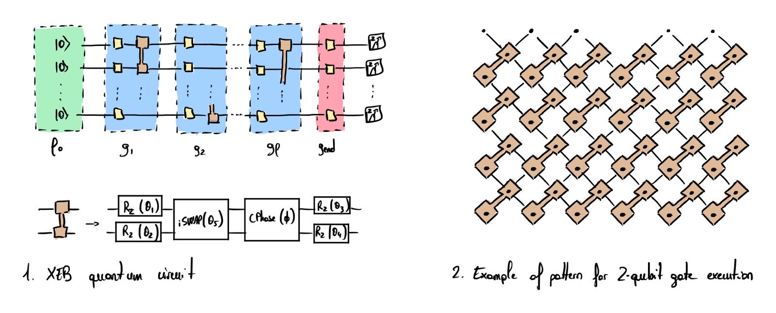
The quantum circuit utilized in this experiment is shown in Fig. 1 and consists of \(l\) layers of quantum gates. Each layer is composed of a wall of single qubit gate uniformly drawn from the set \(\{R_X(\pi/2), R_Y(\pi/2), R_{X+Y}(\pi/2)\}\) (see yellow boxes). Single qubit gates are followed by a set of parallelized two-qubit gates applied according to specific, structured patterns (see Fig. 2 for a pattern example used in the quantum supremacy claim [1]).

The output state is measured in the computational z-basis. For a given random quantum circuit, it is possible—albeit computationally intensive—to calculate the ideal output probability distribution \(\widetilde{p}(x_i)\) of each bitstring \(x_i\) using a classical computer. The classical resources needed for the computation scale exponentially with the number of qubits \(n\). For random circuits, the ideal output probability of each bitstring follows an exponentially decaying distribution, meaning that individual bitstrings are exponentially unlikely to occur as \(n\) increases. However, some bitstrings have higher probabilities than others (e.g. a bitstring might occur with probability \(\frac{2}{2^n}\), others with probability \(\frac{1}{2^n}\) etc…), leading to a non-uniform ideal distribution. If the classical or quantum device fails to sample the output state accurately, the output is supposed to be uncorrelated with the ideal probability distribution. This behavior is detected as the distribution of the output bitstrings being measured will look like a uniform distribution. The central idea behind the XEB protocol is to test whether the quantum processor can generate output bitstrings that exhibit statistically significant correlations with the ideal distribution—thereby deviating from uniformity.

Consider a quantum circuit that implements a random unitary transformation \(U\), i.e., randomly sampled from the Haar measure. The ideal output distribution of this circuit is classically computed and denoted \(\widetilde{p}_U\). The ideal output probability of each bitstring \(x_i\) is then given by \(\widetilde{p}_U(x_i)\). The circuit corresponding to \(U\) is implemented on a quantum computer, and \(k\) samples are realized such that we obtain the set of bitstrings \(S = \{x_1, x_2, ..., x_k\}\). Based on this sample set and the ideal distribution, the following quantity is computed:

If the quantum computer is noisy, the output sampled bitstrings tend to appear independently and identically distributed, meaning that \(\mathbb{E}_i \left[\widetilde{p}_U(x_i) \right] \approx \frac{1}{2^n}\). If the implementation of the quantum computer is ideal, the quantum computer will be able to sample more probable bitstrings with higher probability, which will yield the ideal value \(E_i \left[\widetilde{p}_U(x_i) \right] \approx \frac{2}{2^n}\). This ideal value is valid for all sufficiently deep random quantum circuits. These two bounds form the basis for evaluating quantum performance. In Google’s quantum supremacy experiment, 53 qubits are used to approximately sample \(7,000,000\) bitstrings with multiple random quantum circuits—yielding an empirical value of \(E_i \left[\widetilde{p}_U(x_i) \right] = 1.002\), which exceeds the i.i.d. baseline and thus indicates statistically significant correlation with the ideal distribution. Due to the computational intractability of exactly evaluating \(\widetilde{p}_U(x_i)\) for large size problem, some tricks are used to compute these probabilities (see Supplementary Material of [1] for details).

To ensure statistical significance of the results, a useful rule of thumb is to relate the number of required samples \(k\) to the worst gate fidelity \(\epsilon\) of the quantum processor (\(\epsilon = 0.002\) in the case of Google’s experiment). Specifically, \(k \approx \frac{1}{\epsilon^2}\).

XEB libraries and examples

Some extra references

References

1. [1]S. Boixo et al., “Characterizing quantum supremacy in near-term devices,” Nature Physics, vol. 14, no. 6, pp. 595–600, Apr. 2018, doi: 10.1038/s41567-018-0124-x. [Online]. Available at: http://dx.doi.org/10.1038/s41567-018-0124-x
2. [2]F. Arute et al., “Quantum supremacy using a programmable superconducting processor,” Nature, vol. 574, no. 7779, pp. 505–510, Oct. 2019, doi: 10.1038/s41586-019-1666-5. [Online]. Available at: http://dx.doi.org/10.1038/s41586-019-1666-5