Volumetric Benchmark

Motivation

The Volumetric Benchmark (VB) methodology was proposed in 2019 by R. Blume-Kohout and K. Young from the Sandia National Laboratory in [1]. This methodology generalizes the Quantum Volume proposed earlier by IBM and permits the quantification of a quantum computer’s ability to run a set of circuits successfully. The results are visualized with respect to the width (number of qubits) and depth (number of gates or circuit components in general) of the quantum circuit. The main motivation for this protocol is to extend the quantum volume to rectangular shapes of circuits, as algorithms in the literature do not have the same scaling in depth and width (The authors give an example with Shor’s algorithm, which scales as \(O(n)\) in width and \(O(n^2)\) in depth).

Protocol

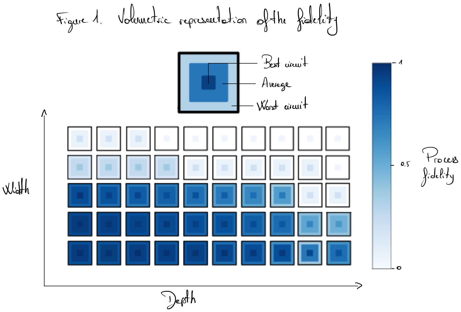
Volumetric benchmark is defined for a set of circuits \(\mathbb{C} = \{C_1, ..., C_l\}\). Each circuit \(C_i\) has an associated width \(w_i\) (number of qubits) and depth \(d_i\). The depth is not restricted to quantum gates; it can also refer to sub-routines (e.g., QFT, Grover oracle) or more complex gates (e.g., multi-control Toffoli gates). A probability distribution may be associated with large sets of circuits if the test does not involve running all the circuits of the set. A criterion of success is defined by the user of the protocol. This criterion defines whether the circuit passes or fails the test. For example, it can be the probability of getting the correct outcome of the circuit \(C_i\) to be beyond a specific threshold. Another example is the average hamming distance between the outcome of the circuit and the true bitstring value (other examples can be found in section 6 of [1]). Further details of experimentation should be specified, such as the compilation process used to run the circuit on a specific hardware or the number of runs for each circuit. A fictional example of benchmarking is shown in Fig. 1. Here, the process fidelity is used as the success metric and extracted from some randomized benchmarking experiment. This fidelity is displayed along with the associated width and depth of the circuit. For each parameter (width and depth), the square displays the fidelity of the best, average, and worst circuit. This graphic representation allows for the display of multiple pieces of information in a compact form. Its purpose is to illustrate the Pareto Frontier (representing the ability of the quantum computer to run the circuits) with respect to the width and depth of quantum circuits.

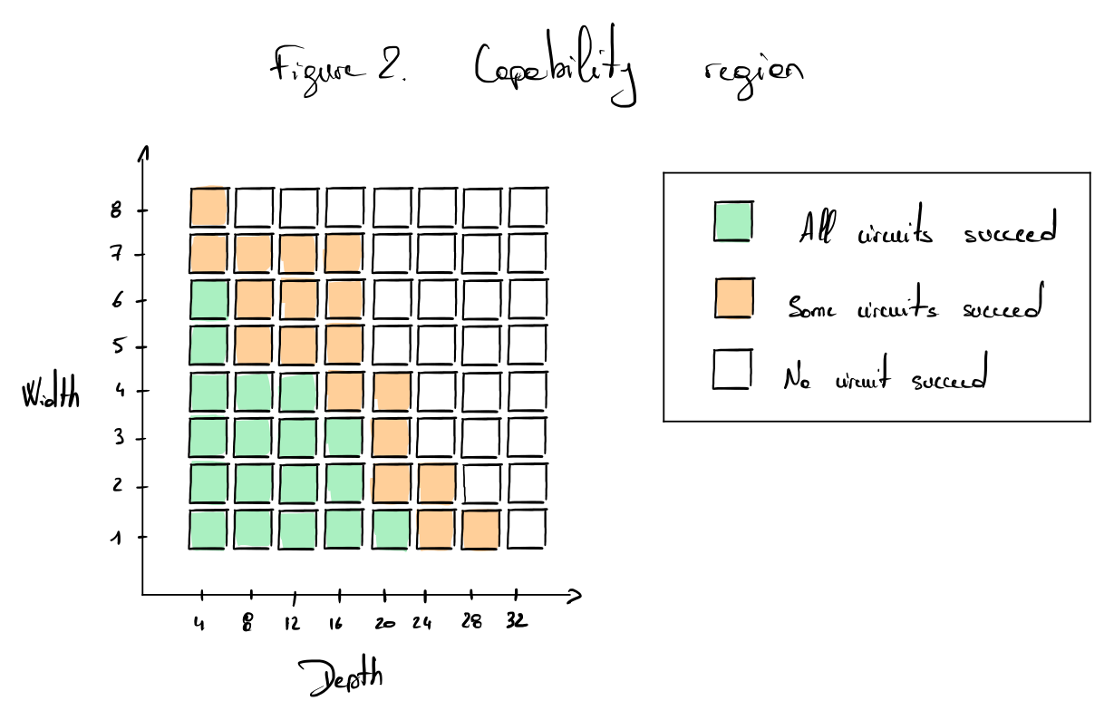
Volumetric benchmark map with the process fidelity (values between 0 and 1) benchmarked along the circuit width and depth.

Using this protocol, it is possible to extract a capability map that clearly outlines the regions where a quantum computer can perform well. An example is shown in Fig. 2.

The volumetric benchmark capability map highlights the regions (combination of width and depth) where the quantum circuit can be run successfully.

Assumptions

The protocol does not impose any rule on several important steps of the benchmark (for example, concerning the compilation process or the possibility of using error mitigation methods). However, it is outlined in [1] that the experimental design should be fairly described.

Limitations

As the experimental design is not strict, comparing results from different studies is impossible, which limits its use in tracking the progress of quantum computer development.
This framework is restricted to quantum circuits; such visualizations are not adapted to benchmark annealing-based solvers.

Implementation

The volumetric benchmark visualization has been implemented in the pyGSTi library, with a tutorial available here.

References

[1]R. Blume-Kohout and K. C. Young, “A volumetric framework for quantum computer benchmarks,” Quantum, vol. 4, p. 362, Nov. 2020, doi: 10.22331/q-2020-11-15-362. [Online]. Available at: http://dx.doi.org/10.22331/q-2020-11-15-362